
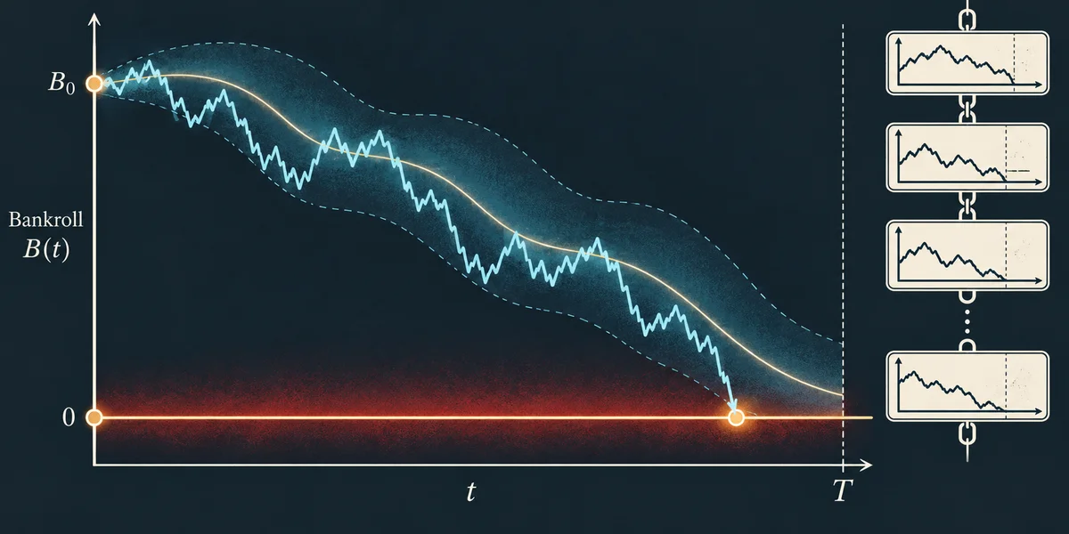

A probability of ruin needs a defined event, a stake rule and a horizon. Reaching zero, lacking the next minimum stake, crossing a chosen loss limit and falling from a previous peak are different events. The same balance path can satisfy some and not others. A percentage without these definitions cannot tell you what risk was calculated, even when it appears beside an advanced theorem.
This article separates three mathematical objects: a discrete fixed-unit walk, a continuous Brownian approximation and an operator risk bound with additional assumptions. It also supplies a funded settlement ledger on the existing synthetic CSV. None is a live study of Lucky Jet or evidence that an operator is solvent. The purpose is to make the inputs and accounting reproducible, while keeping the practical calculator’s actual capabilities clear.
A specified fixed-unit random walk
Begin with independent accepted one-unit bets at a 2x target. Under the declared model, a win has probability p=0.485 and adds one unit; a loss has probability q=0.515 and removes one. There are no fees, new deposits or changing stakes. Integer balance zero is absorbing. A different target generally changes the step sizes: a 1.5x win adds only half a unit, so its chain cannot simply reuse a symmetric-unit formula.
For initial B units and upper stopping wealth M, let R(B) be the probability of zero before reaching M. The boundary conditions are R(0)=1 and R(M)=0. Between them, conditioning on the next outcome gives R(B)=pR(B+1)+qR(B-1). For p≠q, the solution is:
R(B) = ((q/p)^M - (q/p)^B) / ((q/p)^M -1)Here M is a chosen upper wealth boundary, not a measured casino reserve. At B=50, M=100 the ruin-before-doubling probability is about 95.261479%, with success about 4.738521%. These are eventual boundary-hitting probabilities, not the chance of failure within 50 or 100 rounds. They do not say that every person who starts with 50 units will experience that exact outcome.
If the upper boundary is removed and this negative-drift fixed-unit walk continues without replenishment, eventual zero has probability 1. That conclusion belongs to this specified process. It does not establish the same literal-zero event for current-balance fractions, which remain positive on every finite path when their factors are positive and no rounding or minimum applies. Finite-horizon events still need their own calculation.
Finite time changes the question
The discrete process can be computed by tracking mass at every funded balance and retaining zero as absorbed. The finite_bankroll.py reference uses that approach. For the 2x case, it also agrees with an independent first-passage calculation: sum over possible first-zero times n of (B/n)×C(n,(n-B)/2)×p^((n-B)/2)×q^((n+B)/2) , using only matching parity and n≥B.
This formula accounts for paths that hit zero earlier; an ordinary terminal binomial tail would answer a different question. A process can touch the boundary and later recover if it is not stopped, but an absorbing funding rule forbids those later wagers. Likewise, counting a particular losing streak is not the same as counting all paths that reach zero through a mixture of wins and losses.
What the Brownian formula represents
For a separate continuous process X(t)=B+μt+σW(t), with B>0 and σ>0, define τ as the first time X reaches zero. The exact Brownian fixed-barrier distribution for T>0 is:
P(τ ≤ T) = Φ((-B-μT)/(σ√T))
 + exp(-2μB/σ²) Φ((-B+μT)/(σ√T))
Φ denotes the standard normal distribution function. This is a first hit of a fixed zero boundary, not maximum drawdown measured from a moving peak. The University of Chicago lecture on Brownian hitting times gives the corresponding upper-barrier expression; changing the sign of the process yields the lower-barrier form used here.
For the discrete 2x one-unit model, the mean increment is-0.03 and variance is 0.9991. Matching those two moments gives μ=-0.03 and σ²=0.9991 per unit of round time. It does not turn discrete bets into a continuous path. Brownian motion can cross between observation times and has a different increment distribution. The formula is exact for its own process, an approximation when applied to the wager model.
| Initial units | Discrete failure by 1000 | Brownian first-hit approximation |
|---|---|---|
| 20 | 81.337260% | 81.306480% |
| 50 | 37.856629% | 37.799764% |
| 100 | 2.131958% | 2.132118% |
| 250 | 2.306950e-10% | 3.044853e-10% |
The horizon is 1000 rounds in every row. From 100 units the discrete probability is about 2.131958%, rather than an unsupported universal 1.78%. From 250 units both values are extremely small, but the relative difference is material. Agreement at one row does not justify claiming exact accuracy at all bankroll sizes or targets. No row is an empirical frequency from a casino.
The Brownian limits also depend on drift. At μ=0, the expression reduces to 2Φ(-B/(σ√T)). For positive drift, eventual first-hit probability is exp(-2μB/σ²), below 1 but not zero. For negative drift, eventual first hit is certain in this continuous model. Substituting an absolute drift into a positive-drift expression does not create a safety formula for a losing process.
Reproduce both mathematical columns
Save the fixed-unit reference in the same directory as the following Python example. It uses only the standard library and the published helper, with positive bank, variance and horizon inputs. The 4 language versions contain identical executable code. Their discrete and Brownian outputs were run and compared with the displayed table.
# Save finite_bankroll.py in this directory first.
# Fixed one-unit2x model: p=.485, no fees or replenishment.
import json
import logging
import math
from finite_bankroll import fixed_stake_failure

def normal_cdf(z):
    return 0.5 * math.erfc(-z / math.sqrt(2))

def brownian_first_hit(bank, drift, variance, horizon):
    scale = math.sqrt(variance * horizon)
    return (normal_cdf((-bank - drift*horizon) / scale)
            + math.exp(-2*drift*bank/variance)
            * normal_cdf((-bank + drift*horizon) / scale))

rows = []
for bank in [20, 50, 100, 250]:
    rows.append({
        "initialUnits": bank,
        "discreteDp": fixed_stake_failure(bank, 200, 1000),
        "brownianApproximation": brownian_first_hit(bank, -0.03, 0.9991, 1000)
    })
logging.basicConfig(level=logging.INFO, format="%(message)s")
logging.info(json.dumps(rows, indent=2))
Independent checks compared the discrete results with exact rational first-passage sums. The Brownian CDF was also checked against numerical integration of its hitting-time density, including negative, zero and positive drift controls. Those are checks of mathematical implementation. They do not measure a provider’s actual win probability, establish independent live rounds or validate a user’s payment history.
Lundberg’s inequality has conditions
One discrete risk formulation studies independent identically distributed net-loss increments Y, with negative mean loss. A positive adjustment coefficient R must satisfy E[exp(RY)]=1, with the required finite exponential moment. Under the applicable assumptions, an exponential bound controls the chance that cumulative loss exceeds reserve u. The Kent risk-theory notes, chapter 5 state these conditions and the bound.
The result is an upper probability estimate, not a proof that failure is impossible. A positive upper bound is not zero, and positive average income alone does not establish every hypothesis. Correlated liabilities, changing stakes, simultaneous exposure, external costs and an unknown reserve cannot be ignored when discussing a real operator. We have not audited any operator’s accounts or portfolio here.
An unbounded Pareto-type raw multiplier has no finite positive moment-generating function, so the classical positive adjustment-coefficient argument cannot simply be applied to that raw tail. A bounded payment at a fixed accepted cashout is a different random variable. It can have finite exponential moments, but the loss process and its dependence assumptions still need to be specified. Confusing a multiplier with the actual claim paid is the key error to avoid.
A funded replay with three explicit stake rules
Download the existing 10000-round synthetic CSV and ruin_ledgers.py into one directory. Runpython ruin_ledgers.py. The script verifies the file’s documented SHA-256 and reports the following ledger. Add--ledger output.csv if you want every accepted wager for independent inspection. It makes no network calls.
Each replay starts with 1000 units, uses target 2x, counts equality as success and charges no fee. The fixed rules stake 50 or 10. The current rule stakes 0.5% of the settled balance, floors to cents and applies a minimum 0.10. Before each wager it checks funding; it stops before an amount the bank cannot pay. Thus this practical fractional rule differs from the unrounded positive-balance model above.
| Stake rule | Completed wagers | Turnover | Gross payment | Final balance | Realised RTP |
|---|---|---|---|---|---|
| Fixed 50 | 72 | 3600.00 | 2600.00 | 0 | 72.222222% |
| Fixed 10 | 1106 | 11060.00 | 10060.00 | 0 | 90.958409% |
| Current 0.5%, floor cents, min 0.10 | 10000 | 13150.36 | 12200.58 | 50.22 | 92.777536% |
The fixed 50 rule completes 72 wagers, and fixed 10 completes 1106. They reach zero on their last completed wagers; the next intended wagers 73 and 1107 cannot be funded. The fractional rule completes 10000 and ends with 50.22. These are outcomes on one fixed synthetic path, not population failure rates or estimates of average lifespan. The public seeds do not become a predictor of private future rounds.
| Stake rule | First unfunded wager | Maximum peak drawdown |
|---|---|---|
| Fixed 50 | 73 | 100.000000% |
| Fixed 10 | 1107 | 100.000000% |
| Current 0.5%, floor cents, min 0.10 | None in 10000 | 95.396169% |
Maximum drawdown uses every settled point and the highest preceding balance, including the starting amount and final point. The fractional drawdown is approximately 95.396169%, despite never failing its funding check in this file. Ending above zero therefore does not mean avoiding a severe loss. Loss from the initial 1000 alone is 94.978%; the peak-based measure can be larger because the path previously rose or later reached a lower point.
Reconcile the ledger before interpreting it
For each replay, final balance equals initial balance plus gross payouts minus total accepted stakes. Realised RTP equals gross payouts divided by turnover. Fixed 50 has 3600 turnover and 2600 gross, so realised RTP is 72.222222%; fixed 10 has 11060 turnover and 10060 gross, about 90.958409%. The current rule has 13150.36 turnover and 12200.58 gross, about 92.777536%.
All 11178 completed rows were independently checked against the CSV with decimal comparisons, funding checks, integer-cent sums and exact drawdown ratios. SQL totals reproduced stakes and gross payments. These realised returns do not have to equal the declared population 97% on a short or stopped path. Conversely, they do not prove an operator changed its probability law: this is synthetic data with specified rules.
Stopping rules and expected turnover
Under the stated conditional negative-return law, a funded predictable stake S has expected increment-0.03S. For a bounded number of rounds, including a stopping decision, taking expectations gives expected final bank equal to the initial bank minus 0.03 times expected total accepted turnover. The expectation of turnover matters. Substituting one realised stopped turnover is not a conditional prediction of that path’s final balance.
For an unbounded stopping time, theorem conditions such as appropriate integrability cannot be replaced by the phrase “the stop is eventually finite.” A loss limit or profit target can change session-length and outcome distributions without manufacturing positive conditional expectation. A hard spending boundary should be checked before exposing another full stake; a post-settlement stop can overshoot. Simultaneous positions and cashier fees need separate treatment.
Use the tool and references for their actual purpose
The Bankroll Calculator shows unit sizing, model target probability, specified loss sequences, a turnover reference and optional boundaries. It does not provide a full 10000-round survival distribution or Brownian drawdown engine. The offline references make this article reproducible; they do not add those advertised capabilities to the website. The fractional-stake guide explains the separate current-balance model.
No capital ratio here requires increasing an affordable entertainment allocation. Choosing no wager remains valid. Partner actions remain direct registration options with no compulsory demo stage and no guarantee of solvency, available targets or future payment. A useful risk statement names its process, boundary, horizon and evidence. That is more informative than attaching one ruin percentage to every game and every way of staking.